Z-transforms. Bilinear warping. Tustin's method.
What if I told you there's a simpler way to design your loop shaping filters?
📚 Part 4 of the "Control Loop Reality Check" series
- Part 1: The hidden delay that kills your bandwidth
- Part 2: Architecture tricks to fight delay
- Part 3: The lead-lag trick for free gain
Why S-Domain Design Still Works
Remember from Part 1: bandwidth is limited to sample_frequency / 10.
That's actually good news. Your bandwidth is so far below Nyquist that continuous-time design works perfectly—whether you're designing PIDs, lead-lags, notch filters, or any other loop shaping circuit.
The approach is simple: design in the s-domain, then discretize with straightforward integrators. That's it.
All those classic control techniques you learned? Bode plots, frequency response analysis, loop shaping—they all work directly. No warping corrections needed.
The Parametrization Win 🎯
S-domain filters are trivial to parametrize. Your parameters are frequencies in Hz and time constants in seconds—intuitive, physical values:
| Filter Type | S-Domain | Parameters |
|---|---|---|
| Low-pass | $$\frac{1}{s/\omega + 1}$$ | Corner frequency ω |
| Lead-lag | $$\frac{s/\omega_z + 1}{s/\omega_p + 1}$$ | Two corner frequencies |
| Notch filter | $$\frac{s^2 + \omega_n^2}{s^2 + s\omega_n/Q + \omega_n^2}$$ | Center freq + Q |
| Bandpass | $$\frac{s\omega_n/Q}{s^2 + s\omega_n/Q + \omega_n^2}$$ | Center freq + Q |
Try doing that in the z-domain. You'll get ugly exponentials everywhere. Need to change your crossover frequency? Better recalculate everything and verify it still works.
In the s-domain, change sample rate? Your corner frequencies stay put. Your designs remain portable and parametric.
The Integrator That's BETTER Than Analog ✨
You have three main choices for implementing discrete integrators:
| Method | Update Equation |
|---|---|
| Forward Euler | $$y[n] = y[n-1] + T \cdot x[n-1]$$ |
| Backward Euler | $$y[n] = y[n-1] + T \cdot x[n]$$ |
| Trapezoidal | $$y[n] = y[n-1] + \frac{T}{2}(x[n] + x[n-1])$$ |
Here's the surprising part: backward Euler actually beats analog integrators.
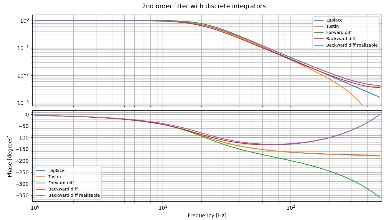
To see why, let's analyze the phase response using $$z = e^{j\omega T}$$:
| Method | Transfer Function | Phase at Nyquist | Verdict |
|---|---|---|---|
| Analog | $$1/s$$ | -90° | Reference |
| Forward Euler | $$\frac{T \cdot z^{-1}}{1 - z^{-1}}$$ | -180° | ❌ Worse! |
| Trapezoidal | $$\frac{T}{2}\frac{1 + z^{-1}}{1 - z^{-1}}$$ | -90° | ≈ Analog |
| Backward Euler | $$\frac{T}{1 - z^{-1}}$$ | 0° | ✅ Free phase margin! |
The backward Euler integrator uses the current input, eliminating the forward delay. At Nyquist where $z^{-1} = -1$:
$$H(e^{j\pi}) = \frac{T}{1-(-1)} = \frac{T}{2}$$
This is a real positive number, giving 0° phase—better than analog's -90°! Forward Euler uses the previous input, introducing a $z^{-1}$ delay that actually makes things worse (-180° at Nyquist).
Stack multiple backward Euler integrators? Each adds another +90° of phase margin at Nyquist. That's bandwidth you didn't know you had.
This isn't a bug. It's a feature.
The Algebraic Loop Problem ⚠️
A backward Euler integrator uses the current input with no delay. When you have overall feedback in a loop, this creates a circular dependency: output depends on input depends on output in the same timestep. The resulting dependency graph has no solution.
Tools like Simulink can't generate code for this because there's no causal ordering of operations. The code generator gets stuck.
Interestingly, forward Euler is the default integrator in Simulink precisely to avoid this problem. Forward Euler uses the previous input x[n-1], which introduces a $z^{-1}$ delay. This breaks the dependency chain, making the computation tractable.
So here's my workflow:
- Design everything with forward Euler first. No algebraic loop errors, easy to debug, straightforward to simulate.
- Once verified, replace the integrators with backward Euler for better phase margin. You lose the algebraic loop protection, but gain superior phase characteristics.
- Add one sample delay in the feedback path. This restores causality, breaking the algebraic loop dependency while keeping your superior backward Euler implementation.
"But we hate delay!" you might say.
Actually, delay placed in the feedback path is slightly better than delay in the forward path. You get marginally less phase shift (at the cost of slightly less attenuation). It's not much, but it's essentially free.
And remember Part 1: we already budgeted one sample of delay into our design. This delay isn't extra—it's expected and already accounted for.
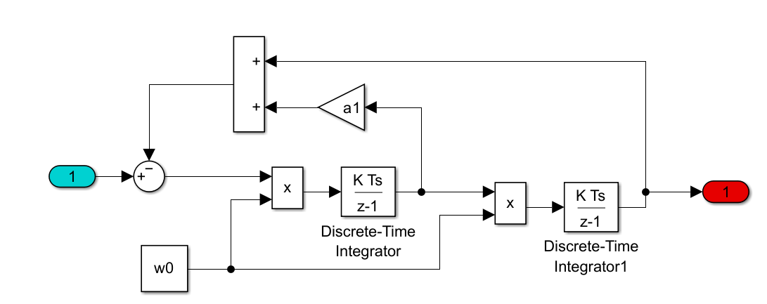
Practical Implementation
Building a digital filter is straightforward once you understand the building blocks. Any s-domain filter is just a combination of gains and integrators:
| Building Block | Implementation | Notes |
|---|---|---|
| Gains | Direct multiply | No issues |
| Integrators (1/s) | Backward Euler | Free phase boost |
| Second order sections | Cascade of integrators | Same benefits apply |
Lead-lags, notch filters, lowpass, bandpass—every one is just a specific arrangement of integrators and gains. Here's what the backward Euler integrator looks like:
# Backward Euler integrator - uses current input for 0° phase at Nyquist
class BackwardEulerIntegrator:
    def __init__(self, dt):
        self.dt = dt
        self.y = 0

    def update(self, x):
        self.y += self.dt * x  # Use CURRENT input
        return self.y
The Recipe
- ✅ Design your loop filter in the s-domain using frequencies in Hz and gains in physical units
- ✅ Implement integrators with backward Euler
- ✅ Add one sample delay in the feedback path to resolve algebraic loops
- ✅ Enjoy the free phase margin at high frequencies—your bandwidth budget increased automatically
Why This Works (The Math)
For a continuous integrator: $$H(s) = \frac{1}{s}$$
The phase at any frequency is -90°.
For backward Euler, the transfer function is:
$$H(z) = \frac{T}{1 - z^{-1}}$$
At Nyquist, substituting $$z = e^{j\pi} = -1$$ so $z^{-1} = -1$:
$$H(e^{j\pi}) = \frac{T}{1 - (-1)} = \frac{T}{2}$$
This is a real positive number, giving 0° phase. Compare that to the analog integrator's -90° at any frequency. The phase climbs back from -90° at DC toward 0° at Nyquist. That's where you get your extra bandwidth.
Summary
| Old Way | New Way |
|---|---|
| Design in z-domain | Design in s-domain |
| Bilinear transform with prewarping | Simple backward Euler |
| Pray the corners are right | Parameters are physical |
| Matched phase to analog | Better phase than analog |
Still wrestling with bilinear transforms? You're working too hard. 💪
Coming Up Next
Part 5: Optimizing loop parameters with a robust optimizer that handles delay—no pole/zero tricks needed. Using the Nyquist criterion geometrically, we can even incorporate measured frequency response data directly. When your plant has delay, standard tools choke. The Nyquist approach just counts crossings.
Questions? War stories about z-domain nightmares? Drop a comment! 👇
#ControlSystems #LoopShaping #DigitalControl #DSP #Embedded