Mathematical models for rectifier circuits with capacitive filtering under two discharge regimes:
- Constant Current: $I_{\text{load}} = \text{constant}$
- Constant Power: $P_{\text{load}} = \text{constant}$
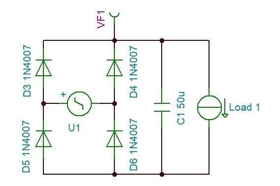
Figure 1: Single-phase full-wave bridge rectifier with capacitive filtering
The implementation defines a minimum voltage threshold $U_{2,\text{min}}$:
$$U_{2,\text{min}} = \begin{cases} U_0 \cos\left(\frac{\pi}{n}\right) & n > 2 \\ 0 & n \leq 2 \end{cases}$$This represents the voltage at the intersection point between adjacent sine waves.
Critical for Constant Power Model:
For the power model, an additional minimum voltage threshold (default 1.0V) must be enforced to prevent physically unrealistic behavior:
Numerical calculations become unstable
Solution: Discharge is forced to stop at $U_{2,\text{min}}$, ensuring:
Physically realistic behavior
Implementation: The solve_U1() method checks if discharge would reach $U_{2,\text{min}}$ and returns this as $U_2$ if it would go lower
Note: This constraint is not needed for the constant current model since $I = \text{const}$ remains finite at all voltages (even at $U = 0$).
AC source period:
$$T = \frac{1}{f}$$Period between charging pulses:
$$T_n = \frac{T}{n} = \frac{1}{nf}$$where $n$ is number of rectification pulses per AC cycle:
- $n=1$: Half-wave single phase
- $n=2$: Full-wave single phase (bridge)
- $n=3$: Three-phase half-wave
- $n=6$: Three-phase full-wave
Angular frequency:
$$\omega = 2\pi f$$Rectified AC voltage:
$$U_{\text{AC}}(t) = U_0 \left|\cos(\omega t)\right|$$Analysis period: $t \in [0, T_n]$
Discharge interval: $t \in [\tau_1, \tau_2]$ where:
- $\tau_1$: discharge start time (diodes turn off) [s]
- $\tau_2$: discharge end time (diodes turn on) [s]
- $U_1 = U(\tau_1)$: voltage at discharge start [V]
- $U_2 = U(\tau_2)$: voltage at discharge end [V]
- $\Delta t = \tau_2 - \tau_1$: discharge duration [s]
Note: In the implementation, $U_1$ is the voltage at $\tau_1$ (start), and $U_2$ is the voltage at $\tau_2$ (end).
Capacitor discharge:
$$I = C\frac{dU}{dt} = -I_{\text{load}}$$Integrating from $\tau_1$ to $t$:
$$U(t) = U_1 - \frac{I_{\text{load}}}{C}(t - \tau_1)$$Voltage at discharge end:
$$U_2 = U_1 - \frac{I_{\text{load}}}{C}\Delta t$$Ripple voltage:
$$\Delta U = U_1 - U_2 = \frac{I_{\text{load}}}{C}\Delta t$$Implementation detail: The discharge is linear between $\tau_1$ and $\tau_2$.
Energy conservation:
$$\frac{1}{2}C U_1^2 - \frac{1}{2}C U^2(t) = P_{\text{load}}(t - \tau_1)$$Solving for $U(t)$:
$$U(t) = \sqrt{U_1^2 - \frac{2P_{\text{load}}}{C}(t - \tau_1)}$$Voltage at discharge end:
$$U_2 = \sqrt{U_1^2 - \frac{2P_{\text{load}}}{C}\Delta t}$$However, $U_2$ is constrained: $U_2 \geq U_{2,\text{min}}$
Ripple voltage:
$$\Delta U = U_1 - U_2$$Critical implementation detail:
The discharge follows a square-root curve, but must be stopped at $U_{2,\text{min}}$ to prevent:
- Infinite current as $U \to 0$ (since $I = P/U$)
- Infinite ripple current in calculations
- Numerical instability
The model enforces $U_2 = \max(\text{calculated } U_2, U_{2,\text{min}})$ where $U_{2,\text{min}}$ is typically 1.0V or higher. This ensures physically realistic behavior by limiting maximum current to $I_{\text{max}} = P/U_{2,\text{min}}$.
Discharge starts when the charging current equals the load current.
Constant current:
Charging current: $I_{\text{charge}} = C\omega U_0 \sin(\omega\tau_1)$
Setting equal to load current:
$$C\omega U_0 \sin(\omega\tau_1) = I_{\text{load}}$$Solving for $\tau_1$:
$$\tau_1 = \frac{1}{\omega}\arcsin\left(\frac{I_{\text{load}}}{C\omega U_0}\right)$$Then $U_1 = U_0\cos(\omega\tau_1)$.
Constant power:
Charging current equals discharge current:
$$\omega C U_0 \sin(\omega\tau_1) = \frac{P_{\text{load}}}{U_0\cos(\omega\tau_1)}$$Simplifying:
$$\omega C U_0^2 \sin(\omega\tau_1)\cos(\omega\tau_1) = P_{\text{load}}$$Using $\sin(2x) = 2\sin(x)\cos(x)$:
$$\sin(2\omega\tau_1) = \frac{2P_{\text{load}}}{\omega C U_0^2}$$Solving for $\tau_1$:
$$\tau_1 = \frac{1}{2\omega}\arcsin\left(\frac{2P_{\text{load}}}{\omega C U_0^2}\right)$$Then $U_1 = U_0\cos(\omega\tau_1)$.
The discharge ends when the capacitor voltage intersects with the next rectified sine wave.
Constant current:
The capacitor voltage must equal the second sine wave:
$$U_0\cos(\omega(T_n - \tau_2)) = U_1 - \frac{I_{\text{load}}}{C}(\tau_2 - \tau_1)$$This is solved numerically using Brent's method by defining:
$$f(U_2) = U_2 - U_1 + \frac{I_{\text{load}}}{C}(\tau_2 - \tau_1)$$where $\tau_2 = T_n - \frac{1}{\omega}\arccos(U_2/U_0)$.
Special case for half-wave (nphase=1): If the capacitor would fully discharge before the next sine wave, then $U_2 = 0$ and $\tau_2 = \tau_1 + U_1 C / I_{\text{load}}$.
Constant power:
Three possible cases:
Intersection with first sine: The discharge curve intersects the descending first sine before reaching the second sine. Solve:
$$U_1^2 - \frac{2P_{\text{load}}}{C}(t - \tau_1) = [U_0\cos(\omega t)]^2$$
Discharge to $U_{2,\text{min}}$: The voltage drops to the minimum threshold before intersecting any sine:
$$\tau_2 = \tau_1 + \frac{C(U_1^2 - U_{2,\text{min}}^2)}{2P_{\text{load}}}$$
Intersection with second sine: The discharge curve intersects the second sine wave. Solve:
$$U_1^2 - \frac{2P_{\text{load}}}{C}(t - \tau_1) = [U_0\cos(\omega(t - T_n))]^2$$
All cases solved numerically using Brent's method.
The discharge curve may intersect the descending first sine before reaching the second sine. This occurs when the discharge is rapid (high power, small capacitance).
The discharge curve $U^2(t) = U_1^2 - \frac{2P_{\text{load}}}{C}(t - \tau_1)$ intersects the first sine $U(t) = U_0\cos(\omega t)$ when:
$$U_1^2 - \frac{2P_{\text{load}}}{C}(t - \tau_1) = [U_0\cos(\omega t)]^2$$Define function:
$$f(t) = U_1^2 - \frac{2P_{\text{load}}}{C}(t - \tau_1) - U_0^2\cos^2(\omega t)$$The implementation checks three scenarios in order:
If $\tau_{2,\text{min}} < \tau_{1,\text{max}}$ (where $\tau_{1,\text{max}} = \frac{1}{\omega}\arccos(U_{2,\text{min}}/U_0)$):
- Use Brent's method to find intersection with first sine
If $\tau_{2,\text{min}} < \tau_{2,\text{min}}$ (where $\tau_{2,\text{min}} = T_n - \tau_{1,\text{max}}$):
- Discharge ends at $U_{2,\text{min}}$ with $\tau_2 = \tau_{2,\text{min}}$
Note: Constant current model cannot intersect the first sine (linear slope is always steeper than cosine descent).
The RMS ripple current has contributions from both charging and discharging phases.
Capacitor current:
$$I_C(t) = \begin{cases} C\omega U_0 \sin(\omega t) & 0 \le t < \tau_1 \text{ (charge)} \\ -I_{\text{load}} & \tau_1 \le t < \tau_2 \text{ (discharge)} \\ C\omega U_0 \sin(\omega(t - T_n)) & \tau_2 \le t < T_n \text{ (charge)} \end{cases}$$RMS ripple current:
$$I_{\text{rms}} = \sqrt{\frac{1}{T_n}\left[\int_0^{\tau_1} I_C^2(t)\,dt + \int_{\tau_1}^{\tau_2} I_C^2(t)\,dt + \int_{\tau_2}^{T_n} I_C^2(t)\,dt\right]}$$Implementation:
def cosint(tau):
    return (w * C * U0)**2 * (tau/2 - sin(2*w*tau)/(4*w))

charging1 = cosint(tau1)
discharging = Iload**2 * (tau2 - tau1)
charging2 = cosint(Tn - tau2_eff)  # tau2_eff handles half-wave case
Iripple = sqrt((charging1 + discharging + charging2) / Tn)
During discharge, current varies as $I = P/U(t)$:
$$I_C^2(t) = \frac{P^2}{U^2(t)} = \frac{P^2}{U_1^2 - \frac{2P}{C}(t-\tau_1)}$$Integrating:
$$\int_{\tau_1}^{\tau_2} \frac{P^2}{U_1^2 - \frac{2P}{C}(t-\tau_1)} dt = CP\ln\left(\frac{U_1}{U_2}\right)$$Critical note: This logarithmic term $\ln(U_1/U_2) \to \infty$ as $U_2 \to 0$, which is why $U_{2,\text{min}}$ is mandatory for the power model. Without it:
- Ripple current calculation diverges
- Numerical integration becomes unstable
- Physical model breaks down (infinite current)
Implementation:
def cosint(tau):
    return (w * C * U0)**2 * (tau/2 - sin(2*w*tau)/(4*w))

charging1 = cosint(tau1)
discharging = C * Pload * log(U1 / U2)
charging2 = cosint(Tn - tau2_eff)
Iripple = sqrt((charging1 + discharging + charging2) / Tn)
Note for half-wave (nphase=1): If $\tau_2 < T_n - T/4$, the capacitor may be empty before the next charging cycle. The implementation uses $\tau_{2,\text{eff}} = \max(\tau_2, T_n - 0.25T)$ to handle this.
Transcendental equations solved using Brent's method (scipy.optimize.brentq):
- Combines bisection with inverse quadratic interpolation
- Guaranteed convergence within bracket
- Efficient for smooth functions
- No derivative required
Constant Current:
1. Check if $I_{\text{load}} > I_{\text{min}}$:
- If yes, capacitor doesn't contribute: return $(\tau_1, U_1, \tau_2, U_2) = (0.5T_n, U_{2,\text{min}}, 0.5T_n, U_{2,\text{min}})$
2. Calculate $\tau_1 = \frac{1}{\omega}\arcsin(I_{\text{load}}/(C\omega U_0))$
3. Calculate $U_1 = U_0\cos(\omega\tau_1)$
4. Check if capacitor fully discharges (half-wave only):
- If $\tau_{\text{empty}} = \tau_1 + U_1 C/I_{\text{load}} \leq T_n - T/4$: return $(\tau_1, U_1, \tau_{\text{empty}}, 0)$
5. Otherwise, solve for $U_2$ using Brent's method:
- Equation: $f(U_2) = U_2 - U_1 + (tau2 - \tau_1)I_{\text{load}}/C = 0$
- Where: $\tau_2 = T_n - \frac{1}{\omega}\arccos(U_2/U_0)$
- Bracket: $[0, U_1]$
6. Calculate $\tau_2$ from $U_2$
7. Calculate $I_{\text{ripple}}$ using ripple_current()
Constant Power:
1. Calculate boundaries: $\tau_{1,\text{max}} = \frac{1}{\omega}\arccos(U_{2,\text{min}}/U_0)$, $\tau_{2,\text{min}} = T_n - \tau_{1,\text{max}}$
2. Check if power is too high: If $\sin(2\omega\tau_1) = \frac{2P}{\omega C U_0^2} \geq 1$:
- Return $(\tau_{1,\text{max}}, U_{2,\text{min}}, \tau_{2,\text{min}}, U_{2,\text{min}})$
3. Calculate $\tau_1 = \frac{1}{2\omega}\arcsin(\frac{2P}{\omega C U_0^2})$
4. If $\tau_1 > \tau_{1,\text{max}}$: return full discharge case
5. Calculate $U_1 = U_0\cos(\omega\tau_1)$
6. Calculate when discharge reaches $U_{2,\text{min}}$: $\tau_{2,U_{2,\text{min}}} = \tau_1 + \frac{C(U_1^2 - U_{2,\text{min}}^2)}{2P}$
7. Case 1: If $\tau_{2,U_{2,\text{min}}} < \tau_{1,\text{max}}$ (intersects first sine):
- Use Brent's method to solve: $f(t) = U_1^2 - \frac{2P}{C}(t-\tau_1) - [U_0\cos(\omega t)]^2 = 0$
- Bracket: $[\tau_{\text{mid}}, 0.5T_n]$ where $\tau_{\text{mid}}$ is adjusted to avoid zero at $\tau_1$
8. Case 2: If $\tau_{2,U_{2,\text{min}}} < \tau_{2,\text{min}}$ (reaches $U_{2,\text{min}}$ between sines):
- Return $(\tau_1, U_1, \tau_{2,U_{2,\text{min}}}, U_{2,\text{min}})$
9. Case 3: Otherwise (intersects second sine):
- Use Brent's method to solve: $f(t) = U_1^2 - \frac{2P}{C}(t-\tau_1) - [U_0\cos(\omega(t-T_n))]^2 = 0$
- Bracket: $[T_n/2, T_n]$
10. Calculate $I_{\text{ripple}}$ using ripple_current()
Constant current (for specified ripple $\Delta U = U_1 - U_2$):
$$C \geq \frac{I_{\text{load}}\Delta t}{\Delta U}$$For small ripple approximation where $\Delta t \approx T_n$:
$$C \geq \frac{I_{\text{load}}}{nf\Delta U}$$Constant power (for specified ripple $\Delta U = U_1 - U_2$):
Exact:
$$C = \frac{2P_{\text{load}}\Delta t}{U_1^2 - U_2^2}$$Small ripple approximation where $U_1 \approx U_2 \approx \bar{U}$:
$$C \geq \frac{P_{\text{load}}}{nf\bar{U}\Delta U}$$where $\bar{U} = \frac{U_1 + U_2}{2}$ is the average voltage.
Constant current:
For the capacitor to contribute to smoothing:
$$I_{\text{load}} < I_{\text{min}} = C\omega U_0 \sin\left(\frac{\pi}{n}\right)$$If this condition is violated, the output voltage drops to $U_{2,\text{min}}$.
Constant power:
For the discharge not to reach $U_{2,\text{min}}$:
$$\sin(2\omega\tau_1) = \frac{2P_{\text{load}}}{\omega C U_0^2} < 1$$This gives:
$$C > \frac{2P_{\text{load}}}{\omega U_0^2} = \frac{P_{\text{load}}}{\pi f U_0^2}$$| Property | Constant Current | Constant Power |
|---|---|---|
| Equation | $U(t) = U_1 - \frac{I}{C}(t-\tau_1)$ | $U(t) = \sqrt{U_1^2 - \frac{2P}{C}(t-\tau_1)}$ |
| Shape | Linear | Curved (square root) |
| Current | $I = \text{const}$ | $I = P/U(t)$ (increases as $U$ drops) |
| Current limit | Finite at all voltages | $I \to \infty$ as $U \to 0$ |
| U2_min constraint | Not required | Required (prevents infinite current) |
| End voltage | $U_2 = U_1 - \frac{I}{C}\Delta t$ | $U_2 = \max(\sqrt{U_1^2 - \frac{2P}{C}\Delta t}, U_{2,\text{min}})$ |
| First sine intersection? | No | Yes (possible) |
| Minimum voltage | Can reach 0 (half-wave) | Limited by $U_{2,\text{min}}$ (typically 1.0V) |
| Finding $\tau_1$ | $\arcsin(I/(C\omega U_0))$ | $\arcsin(2P/(C\omega U_0^2))/2$ |
| Finding $\tau_2$ | Brent's method + special case | Brent's method + 3 cases |
Key difference: The power model requires $U_{2,\text{min}}$ because without it, current $I=P/U$ becomes infinite as voltage approaches zero, causing ripple current calculations ($\propto \ln(U_1/U_2)$) to diverge and making the model physically unrealistic.
Constant current:
$$E = \int_{\tau_1}^{\tau_2} U(t)I\,dt = I\int_{\tau_1}^{\tau_2} \left(U_1 - \frac{I}{C}(t-\tau_1)\right)dt$$ $$E = I\Delta t\left(U_1 - \frac{I\Delta t}{2C}\right) = I\Delta t\cdot\frac{U_1 + U_2}{2}$$Constant power:
$$E = P\Delta t = \frac{1}{2}C(U_1^2 - U_2^2)$$The implementation uses an object-oriented design with a base class and two derived classes:
RectifierModelBase(ABC) - Abstract base classRectifierModelCurrent(RectifierModelBase) - Constant current discharge modelRectifierModelPower(RectifierModelBase) - Constant power discharge model# Constant current model
rm = RectifierModelCurrent(T, nphase, U0)
# Constant power model
rm = RectifierModelPower(T, nphase, U0, U2_min=1.0)
Parameters:
- T: Period time of sine [s]
- nphase: Number of rectification pulses per AC cycle
- U0: Rectified sine amplitude [V]
- U2_min: Minimum voltage threshold [V] (power model only, default=1.0)
solve_U1(C, load_param) -> (tau1, U1, tau2, U2)Calculate discharge curve parameters for given capacitance and load.
Parameters:
- C: Capacitance [F]
- load_param: Load current [A] for current model, or Load power [W] for power model
Returns:
- tau1: Discharge start time [s]
- U1: Voltage at discharge start [V]
- tau2: Discharge end time [s]
- U2: Voltage at discharge end [V]
ripple_current(tau1, tau2, C, load_param) -> IrippleCalculate RMS ripple current.
Parameters:
- tau1, tau2: Discharge times [s]
- C: Capacitance [F]
- load_param: Load current [A] or power [W]
Returns:
- Iripple: RMS ripple current [A]
build_discharge_waveform(C, load_param, npoints) -> (tt, sinewave, capwave, tau1, U1, tau2, U2)Build complete voltage waveform for one period.
Parameters:
- C: Capacitance [F]
- load_param: Load current [A] or power [W]
- npoints: Number of sample points
Returns:
- tt: Time array [s]
- sinewave: Sine envelope voltage [V]
- capwave: Capacitor/output voltage [V]
- tau1, U1, tau2, U2: Discharge parameters
build_U1_ripple(Cmax, load_param, npoints) -> (cc, uu1, irr)Build arrays of U1 and ripple current vs capacitance.
Parameters:
- Cmax: Maximum capacitance [F]
- load_param: Load current [A] or power [W]
- npoints: Number of capacitance points
Returns:
- cc: Capacitance array [F]
- uu1: U1 voltage array [V]
- irr: Ripple current array [A]
compute_fft_spectrum(C, load_param, n_samples=4096) -> dictCompute FFT spectrum of the discharge waveform.
Parameters:
- C: Capacitance [F]
- load_param: Load current [A] or power [W]
- n_samples: Number of FFT samples (power of 2 recommended)
Returns: Dictionary with keys:
- 'frequencies': Frequency array [Hz]
- 'magnitudes': Magnitude array [V]
- 'phases': Phase array [rad]
- 'dc_component': DC voltage [V]
- 'thd': Total Harmonic Distortion [%]
- 'harmonics': List of (harmonic_number, frequency, magnitude, magnitude_percent)
- 'waveform': Voltage waveform [V]
- 'time': Time array [s]
get_model_name() -> str: Returns "Constant Current" or "Constant Power"get_model_description() -> str: Returns usage descriptionget_discharge_type() -> str: Returns "Linear" or "Non-linear (square root)"get_load_param_name() -> str: Returns "Load Current" or "Load Power"get_load_param_unit() -> str: Returns "A" or "W"get_load_param_description() -> str: Returns parameter descriptionimport numpy as np
from pages.rectifier.rectifier_current import RectifierModelCurrent
# Create model for 50Hz, full-wave bridge rectifier, 325V peak
rm = RectifierModelCurrent(T=1/50, nphase=2, U0=325)
# Analyze with 100μF capacitor, 1A load
C = 100e-6
Iload = 1.0
# Get discharge parameters
tau1, U1, tau2, U2 = rm.solve_U1(C, Iload)
Iripple = rm.ripple_current(tau1, tau2, C, Iload)
print(f"Discharge start: τ1={tau1*1000:.3f}ms, U1={U1:.1f}V")
print(f"Discharge end: τ2={tau2*1000:.3f}ms, U2={U2:.1f}V")
print(f"Voltage ripple: ΔU={U1-U2:.1f}V")
print(f"Ripple current: Irms={Iripple:.3f}A")
# Build waveform
tt, sinewave, capwave, tau1, U1, tau2, U2 = rm.build_discharge_waveform(C, Iload, npoints=1000)
# Analyze frequency content
fft_data = rm.compute_fft_spectrum(C, Iload)
print(f"DC component: {fft_data['dc_component']:.2f}V")
print(f"THD: {fft_data['thd']:.2f}%")
The model makes several idealizing assumptions:
Diode forward voltage drops:
The model assumes ideal diodes ($V_{\text{diode}} = 0$). To account for real diode voltage drops:
Half-wave rectifier (1 diode): Subtract one diode drop from peak voltage
$$U_0 = U_{\text{peak,AC}} - V_{\text{diode}}$$
Full-wave bridge (2 diodes in series): Subtract two diode drops
$$U_0 = U_{\text{peak,AC}} - 2V_{\text{diode}}$$
Three-phase rectifiers: Subtract appropriate number of diode drops in conduction path
Typical diode forward voltages:
- Silicon diodes: $V_{\text{diode}} \approx 0.7$ V (low current) to $1.0$ V (high current)
- Schottky diodes: $V_{\text{diode}} \approx 0.3$ V to $0.5$ V
- High-voltage rectifiers: $V_{\text{diode}} \approx 1.0$ V to $1.5$ V
Example: For 230V AC RMS (325V peak) with bridge rectifier using silicon diodes:
$$U_0 = 325\text{ V} - 2 \times 1.0\text{ V} = 323\text{ V}$$Other real-world effects to consider:
- ESR (Equivalent Series Resistance): Causes additional voltage drop proportional to ripple current, reduces effective capacitance
- Charging time: Real diodes and wiring have finite impedance, charging is not instantaneous
- Load variations: Real loads may vary with voltage or time (not perfectly constant)
- AC source quality: Mains voltage may contain harmonics, distortion, or frequency variations
For high-precision applications, these effects should be characterized experimentally or with detailed circuit simulation.
The output voltage waveform is periodic with fundamental ripple frequency:
$$f_{\text{ripple}} = nf$$The waveform can be decomposed into DC component and harmonics:
$$U(t) = U_{\text{DC}} + \sum_{k=1}^{\infty} A_k \cos(2\pi k f_{\text{ripple}} t + \phi_k)$$where:
- $U_{\text{DC}}$ = average voltage
- $A_k$ = amplitude of $k$-th harmonic
- $\phi_k$ = phase of $k$-th harmonic
The implementation uses scipy.fft.rfft for real-valued FFT on one period $T_n$:
Algorithm:
1. Build discharge waveform using build_discharge_waveform(C, load_param, n_samples)
2. Compute FFT: fft_result = scipy.fft.rfft(capwave)
3. Get frequencies: frequencies = scipy.fft.rfftfreq(n_samples, dt)
4. Calculate magnitudes: magnitudes = abs(fft_result) * 2.0 / n_samples
5. DC component: dc_component = magnitudes[0] / 2.0 (DC is not doubled)
Harmonic identification:
- Fundamental frequency: $f_{\text{ripple}} = n/T$
- For each harmonic $k = 1, 2, ..., 20$:
- Find frequency bin closest to $k \cdot f_{\text{ripple}}$
- Extract magnitude and compute percentage of DC
THD calculation:
$$\text{THD} = \frac{\sqrt{\sum_{k=2}^{20} A_k^2}}{A_1} \times 100\%$$where $A_1$ is the fundamental ripple component (k=1), and harmonics 2-20 are summed.